Simpson's Paradox: An Example
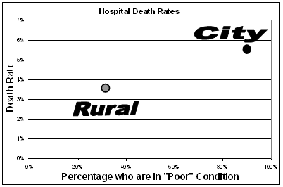
Consider the percentage of
patients who die at two hospitals: City and Rural. As shown in the
graph on the left, the patient death rate is higher at City (5.5%) than
at Rural (3.%). While one might infer that Rural is the
better hospital, association does not prove causation. An
alternate explanation is the difference in mixture of patients in poor
condition. At City, 90% are in poor condition while at the Rural
hospital only 30% are in poor condition.
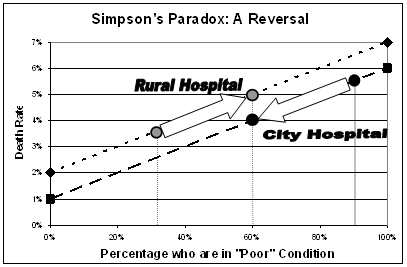
The graph on the right
clearly shows that patients in poor condition have a higher death rate
than other patients.
Among patients in poor
condition (on the right side), the death rate is 7% at the Rural
hospital and 6% at the City hospital. Among patients not in poor
condition (on the left side), the death rate is 2% at the Rural hospital
and 1% at the City hospital. The diagonal lines are the weighted
average lines. The average reflects the mixture of the two groups.
The 5.5% average death rate at city hospital reflects the fact that 90%
of the city patients are in poor condition. The 3.5% average death
rate at rural hospital reflects the fact that only 30% of the rural
hospital patients are in poor condition.
 
What would the death rates be if both hospitals had the same mix of patients?
We need
to standardize: to recalculate the death rates using the same mix of
patients.
Suppose that for both hospitals combined, 60% of all
patients were in poor condition. Suppose we gave each hospital
this same mix.
Note that we are not changing the death rates for any subgroup -- we are
just changing the mixture of the subgroups.
In
that case, the average death rate at the City hospital would decrease while the
average death rate at the rural hospital would increase.
And in this particular case,
they reversed. The standardized death rate is higher for
Rural than for City.
This reversal is Simpson's
Paradox. The difference in mix is confounded (tangled up) with the
difference in death rates for the two hospitals. Standardizing is
one way to untangle the influence of a binary confounder.
Standardizing Interactively On-Line
On-line interactive
versions of this standardizing technique are available.
Changing the
data changes the standardized values in the graph.
General
Articles on Simpson's Paradox:
Simpson's Paradox and Cornfield's Conditions (1999)
by Milo Schield, Augsburg College,
Director of the W. M. Keck Statistical Literacy Project
Abstract: Simpson's
Paradox occurs when an observed association is spurious – reversed
after taking into account a confounding factor. At best, Simpson's
Paradox is used to argue that association is not causation. At
worst, Simpson's Paradox is used to argue that induction is
impossible in observational studies (that all arguments from
association to causation are equally suspect) since any association
could possibly be reversed by some yet unknown confounding factor.
This paper reviews Cornfield's conditions – the necessary conditions
for Simpson's Paradox – and argues that a simple-difference form of
these conditions can be used to establish a minimum effect size for
any potential confounder. Cornfield's minimum effect size is
asserted to be a key element in statistical literacy. In order to
teach this important concept, a graphical technique was developed to
illustrate percentage-point difference comparisons. Some preliminary
results of teaching these ideas in an introductory statistics course
are presented.
Three Graphs to
Promote Statistical Literacy (2004)
by Milo Schield, Augsburg College,
Director of the W. M. Keck Statistical Literacy Project
Abstract: Graphical techniques
have been used in introductory statistics to teach three big
statistical topics: (1) confounding (which can result in Simpson’s
Paradox), (2) statistical significance and (3) the vulnerability of
statistical significance to confounding. These graphical techniques
have been used to teach students as part of the W. M. Keck
Statistical Literacy project. These graphs have transformed
statistical education at Augsburg College; they can change
statistical education everywhere.
Real-World Examples of Simpson's Paradox:
Instance of Simpson's Paradox in NAEP Data
(thanks to David Stein and Bob Hayden) [Broken link
12/08]
Frequency of Simpson's Paradox in NAEP Data (4/2004)
by James
Terwilliger (NAEP Coordinator, Minnesota Department of Education)
and Milo Schield, Augsburg College,
Director of the W. M. Keck Statistical Literacy Project
Abstract (extract): In state education data, Simpson’s
Paradox occurs for two states when their difference in scores has the
opposite sign of the score differences for each of the state subgroups.
Simpson’s Paradox is a specific manifestation of statistical
confounding. The paradox has been understood for many years but is
usually regarded as simply a curious anomaly.
The purpose of this paper is to
show that Simpson’s Paradox is not rare in NAEP data. NAEP public-school data are
analyzed for 2000n Grade 4 Math and 2002 Grade 8 Reading. Approximately
100 instances of Simpson’s Paradox are found per data set based on the
influence of three confounders: family income, school location and
race/ethnicity.
As a percentage of all pairs of
state differences in the same data that are statistically significant,
4% are reversed using a conservative approach while 10% are reversed
using a more liberal approach. All Simpson’s reversals – whether
statistically significant or not – are argued to have ‘journalistic
significance’ because of their political significance. The failure to
allow adjustments for confounders can lead to a serious
misinterpretation of the results which in turn can lead to questionable
policies.
Links involving Simpson's Paradox:
Articles Involving the Cornfield Conditions:
- Wikipedia:
Simpson's
Paradox
- Ding, P., & Vanderweele, T.
(2014). Generalized cornfield conditions for the risk difference.
Biometrika, 101, 1–13.
- Ding, P., & Vanderweele, T.
(2016). Sensitivity analysis without assumptions. Epidemiology, 27,
368–377.
- Ding, P., & VanderWeele, T.
(2017). Sensitivity analysis in observational research: Introducing
the E-value. Annals of Internal Medicine, 167(4), 268–274.
Examples of Simpson's Paradox
Articles involving Simpson's Paradox:
- Blyth, CR (1972) On Simpson's Paradox and the Sure-Thing
Principle. 1972 Journal of the American Statistical
Association 67(338):364-366. DOI10.2307/2284382
- Samuels, Myra L. (1993). Simpson's Paradox and Related
Phenomena. Journal of the American Statistical Association Volume
88, 1993 - Issue 421 Published online: 20 Dec 2012
- Pearl, Judea (2014). Comment: Understanding Simpson’s Paradox.
Pages 8-13 Published online: 21 Feb 2014,
|


